Prior Probability Distributions
Selection and Discrimination

University of Victoria
2025-07-29
Sample code
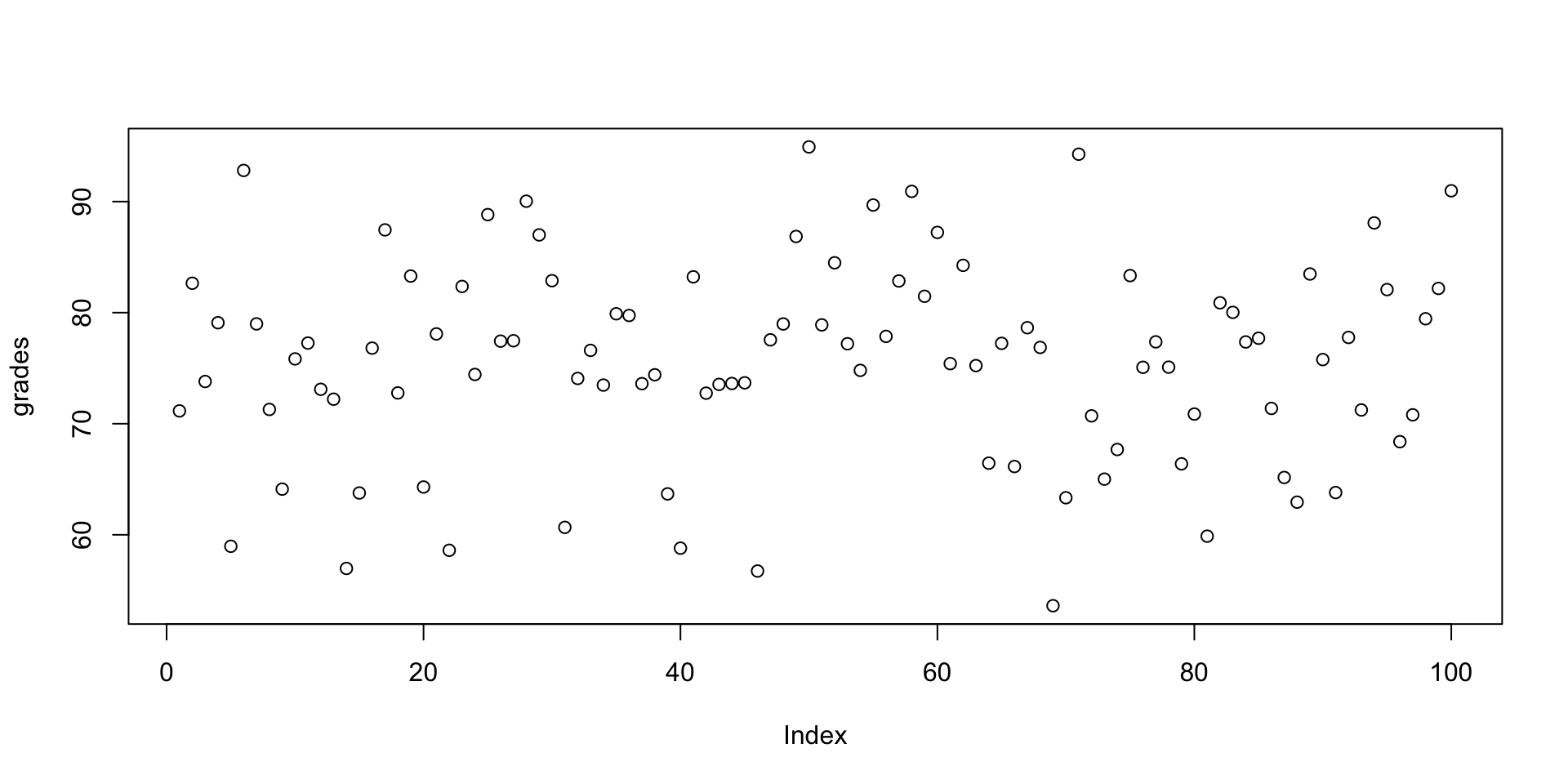
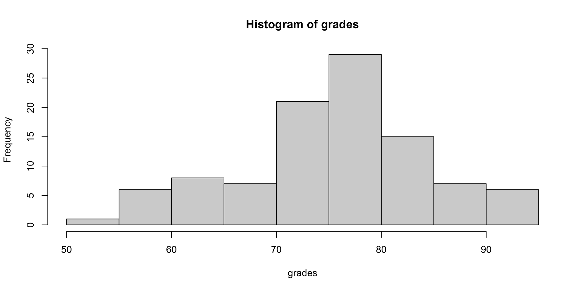
and get a vector of grades, again randomly distributed according to the parameterization we specified. (Hmm, new grading idea!)
Playing with Distributions
Code
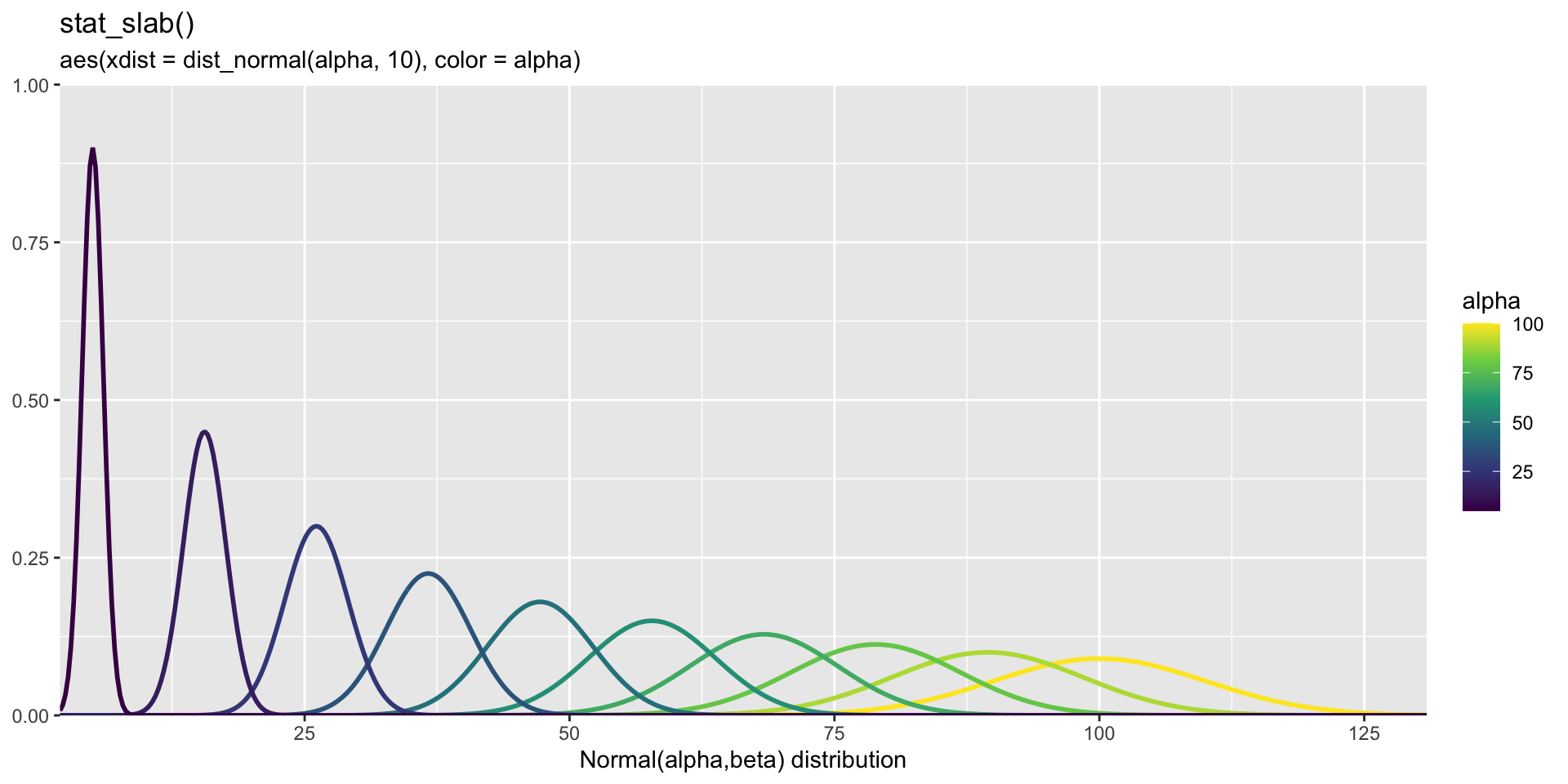
library(ggdist)
library(distributional)
data.frame(alpha = seq(5, 100, length.out = 10), beta = seq(1,10,length.out=10)) %>%
  ggplot(aes(xdist = dist_normal(mu=alpha, sigma=beta), color = alpha)) +
  stat_slab(fill = NA) +
  coord_cartesian(expand = FALSE) +
  scale_color_viridis_c() +
  labs(
    title = "stat_slab()",
    subtitle = "aes(xdist = dist_normal(alpha, 10), color = alpha)",
    x = "Normal(alpha,beta) distribution",
    y = NULL
  )
Code
Code
par(mfrow = c(1, 1), mar = c(4, 4, 2, 1))
plot.legend <- c("Weibull", "lognormal", "gamma")
# three different distributions we can check
fw <- fitdist(groundbeef$serving, "weibull")
fg <- fitdist(groundbeef$serving, "gamma")
fln <- fitdist(groundbeef$serving, "lnorm")
denscomp(list(fw, fln, fg), legendtext = plot.legend)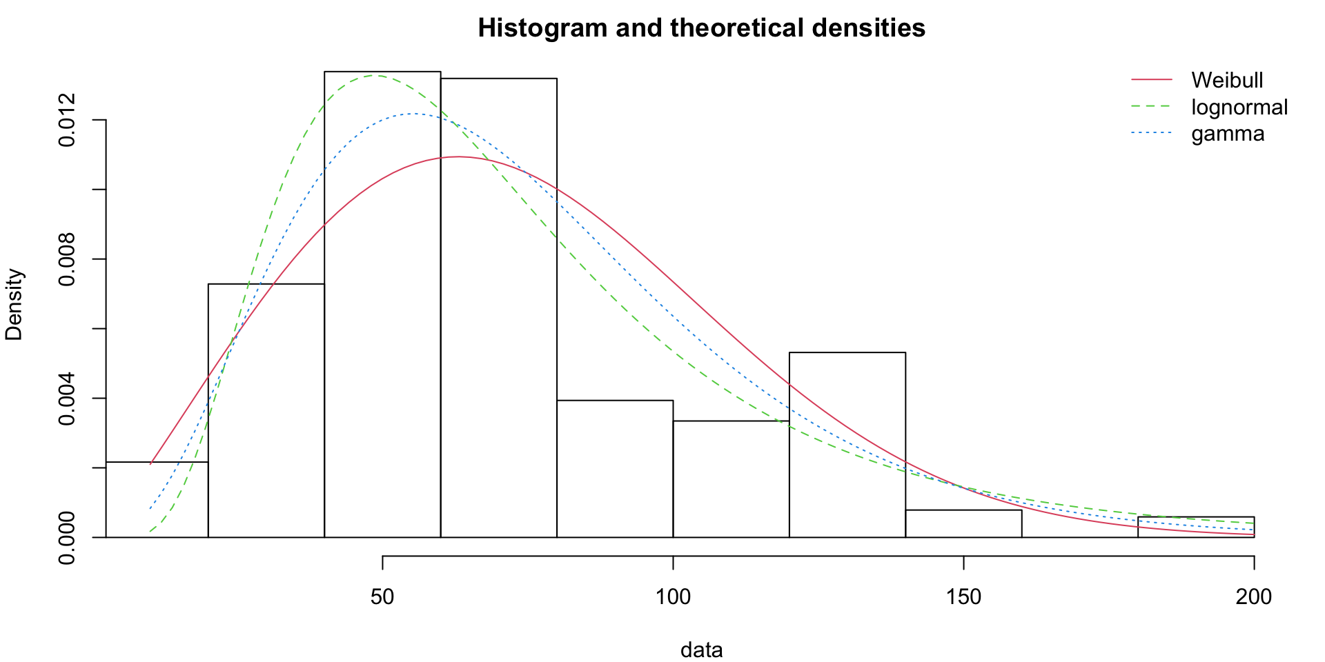
Weakly-informative, Uninformative, Opionated
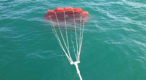
A prior acts like a sea anchor or drogue chute on the engine of the data and likelihood.
Here’s a sea anchor:
SAMPLING FOR MODEL 'continuous' NOW (CHAIN 1).
Chain 1:
Chain 1: Gradient evaluation took 5.7e-05 seconds
Chain 1: 1000 transitions using 10 leapfrog steps per transition would take 0.57 seconds.
Chain 1: Adjust your expectations accordingly!
Chain 1:
Chain 1:
Chain 1: Iteration:    1 / 2000 [  0%]  (Warmup)
Chain 1: Iteration:  200 / 2000 [ 10%]  (Warmup)
Chain 1: Iteration:  400 / 2000 [ 20%]  (Warmup)
Chain 1: Iteration:  600 / 2000 [ 30%]  (Warmup)
Chain 1: Iteration:  800 / 2000 [ 40%]  (Warmup)
Chain 1: Iteration: 1000 / 2000 [ 50%]  (Warmup)
Chain 1: Iteration: 1001 / 2000 [ 50%]  (Sampling)
Chain 1: Iteration: 1200 / 2000 [ 60%]  (Sampling)
Chain 1: Iteration: 1400 / 2000 [ 70%]  (Sampling)
Chain 1: Iteration: 1600 / 2000 [ 80%]  (Sampling)
Chain 1: Iteration: 1800 / 2000 [ 90%]  (Sampling)
Chain 1: Iteration: 2000 / 2000 [100%]  (Sampling)
Chain 1:
Chain 1:  Elapsed Time: 0.014 seconds (Warm-up)
Chain 1:                0.014 seconds (Sampling)
Chain 1:                0.028 seconds (Total)
Chain 1:

SAMPLING FOR MODEL 'continuous' NOW (CHAIN 2).
Chain 2:
Chain 2: Gradient evaluation took 3e-06 seconds
Chain 2: 1000 transitions using 10 leapfrog steps per transition would take 0.03 seconds.
Chain 2: Adjust your expectations accordingly!
Chain 2:
Chain 2:
Chain 2: Iteration:    1 / 2000 [  0%]  (Warmup)
Chain 2: Iteration:  200 / 2000 [ 10%]  (Warmup)
Chain 2: Iteration:  400 / 2000 [ 20%]  (Warmup)
Chain 2: Iteration:  600 / 2000 [ 30%]  (Warmup)
Chain 2: Iteration:  800 / 2000 [ 40%]  (Warmup)
Chain 2: Iteration: 1000 / 2000 [ 50%]  (Warmup)
Chain 2: Iteration: 1001 / 2000 [ 50%]  (Sampling)
Chain 2: Iteration: 1200 / 2000 [ 60%]  (Sampling)
Chain 2: Iteration: 1400 / 2000 [ 70%]  (Sampling)
Chain 2: Iteration: 1600 / 2000 [ 80%]  (Sampling)
Chain 2: Iteration: 1800 / 2000 [ 90%]  (Sampling)
Chain 2: Iteration: 2000 / 2000 [100%]  (Sampling)
Chain 2:
Chain 2:  Elapsed Time: 0.013 seconds (Warm-up)
Chain 2:                0.012 seconds (Sampling)
Chain 2:                0.025 seconds (Total)
Chain 2:

SAMPLING FOR MODEL 'continuous' NOW (CHAIN 3).
Chain 3:
Chain 3: Gradient evaluation took 2e-06 seconds
Chain 3: 1000 transitions using 10 leapfrog steps per transition would take 0.02 seconds.
Chain 3: Adjust your expectations accordingly!
Chain 3:
Chain 3:
Chain 3: Iteration:    1 / 2000 [  0%]  (Warmup)
Chain 3: Iteration:  200 / 2000 [ 10%]  (Warmup)
Chain 3: Iteration:  400 / 2000 [ 20%]  (Warmup)
Chain 3: Iteration:  600 / 2000 [ 30%]  (Warmup)
Chain 3: Iteration:  800 / 2000 [ 40%]  (Warmup)
Chain 3: Iteration: 1000 / 2000 [ 50%]  (Warmup)
Chain 3: Iteration: 1001 / 2000 [ 50%]  (Sampling)
Chain 3: Iteration: 1200 / 2000 [ 60%]  (Sampling)
Chain 3: Iteration: 1400 / 2000 [ 70%]  (Sampling)
Chain 3: Iteration: 1600 / 2000 [ 80%]  (Sampling)
Chain 3: Iteration: 1800 / 2000 [ 90%]  (Sampling)
Chain 3: Iteration: 2000 / 2000 [100%]  (Sampling)
Chain 3:
Chain 3:  Elapsed Time: 0.013 seconds (Warm-up)
Chain 3:                0.016 seconds (Sampling)
Chain 3:                0.029 seconds (Total)
Chain 3:

SAMPLING FOR MODEL 'continuous' NOW (CHAIN 4).
Chain 4:
Chain 4: Gradient evaluation took 2e-06 seconds
Chain 4: 1000 transitions using 10 leapfrog steps per transition would take 0.02 seconds.
Chain 4: Adjust your expectations accordingly!
Chain 4:
Chain 4:
Chain 4: Iteration:    1 / 2000 [  0%]  (Warmup)
Chain 4: Iteration:  200 / 2000 [ 10%]  (Warmup)
Chain 4: Iteration:  400 / 2000 [ 20%]  (Warmup)
Chain 4: Iteration:  600 / 2000 [ 30%]  (Warmup)
Chain 4: Iteration:  800 / 2000 [ 40%]  (Warmup)
Chain 4: Iteration: 1000 / 2000 [ 50%]  (Warmup)
Chain 4: Iteration: 1001 / 2000 [ 50%]  (Sampling)
Chain 4: Iteration: 1200 / 2000 [ 60%]  (Sampling)
Chain 4: Iteration: 1400 / 2000 [ 70%]  (Sampling)
Chain 4: Iteration: 1600 / 2000 [ 80%]  (Sampling)
Chain 4: Iteration: 1800 / 2000 [ 90%]  (Sampling)
Chain 4: Iteration: 2000 / 2000 [100%]  (Sampling)
Chain 4:
Chain 4:  Elapsed Time: 0.013 seconds (Warm-up)
Chain 4:                0.013 seconds (Sampling)
Chain 4:                0.026 seconds (Total)
Chain 4: Priors for model 'weak_prior_test'
------
Intercept (after predictors centered)
Specified prior:
~ normal(location = 20, scale = 2.5)
Adjusted prior:
~ normal(location = 20, scale = 15)
Coefficients
Specified prior:
~ normal(location = 0, scale = 2.5)
Adjusted prior:
~ normal(location = 0, scale = 15)
Auxiliary (sigma)
Specified prior:
~ exponential(rate = 1)
Adjusted prior:
~ exponential(rate = 0.17)
------
See help('prior_summary.stanreg') for more details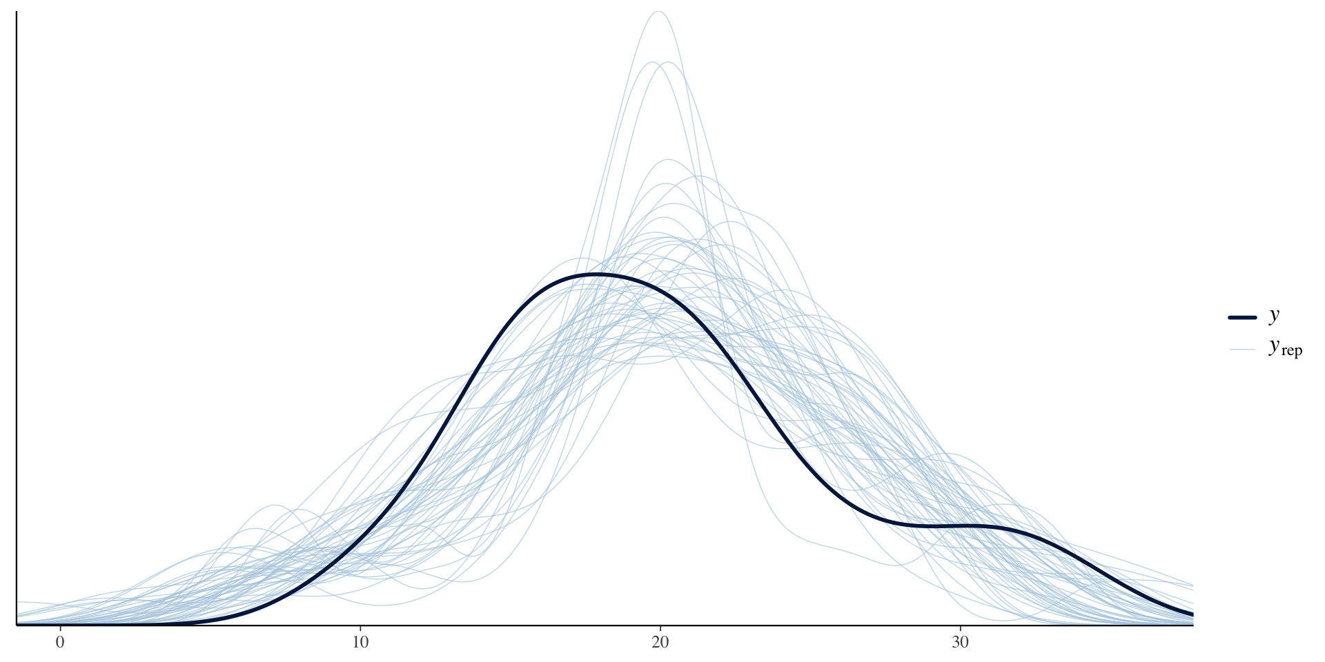
SAMPLING FOR MODEL 'continuous' NOW (CHAIN 1).
Chain 1:
Chain 1: Gradient evaluation took 1.3e-05 seconds
Chain 1: 1000 transitions using 10 leapfrog steps per transition would take 0.13 seconds.
Chain 1: Adjust your expectations accordingly!
Chain 1:
Chain 1:
Chain 1: Iteration:    1 / 2000 [  0%]  (Warmup)
Chain 1: Iteration:  200 / 2000 [ 10%]  (Warmup)
Chain 1: Iteration:  400 / 2000 [ 20%]  (Warmup)
Chain 1: Iteration:  600 / 2000 [ 30%]  (Warmup)
Chain 1: Iteration:  800 / 2000 [ 40%]  (Warmup)
Chain 1: Iteration: 1000 / 2000 [ 50%]  (Warmup)
Chain 1: Iteration: 1001 / 2000 [ 50%]  (Sampling)
Chain 1: Iteration: 1200 / 2000 [ 60%]  (Sampling)
Chain 1: Iteration: 1400 / 2000 [ 70%]  (Sampling)
Chain 1: Iteration: 1600 / 2000 [ 80%]  (Sampling)
Chain 1: Iteration: 1800 / 2000 [ 90%]  (Sampling)
Chain 1: Iteration: 2000 / 2000 [100%]  (Sampling)
Chain 1:
Chain 1:  Elapsed Time: 0.014 seconds (Warm-up)
Chain 1:                0.014 seconds (Sampling)
Chain 1:                0.028 seconds (Total)
Chain 1:

SAMPLING FOR MODEL 'continuous' NOW (CHAIN 2).
Chain 2:
Chain 2: Gradient evaluation took 5e-06 seconds
Chain 2: 1000 transitions using 10 leapfrog steps per transition would take 0.05 seconds.
Chain 2: Adjust your expectations accordingly!
Chain 2:
Chain 2:
Chain 2: Iteration:    1 / 2000 [  0%]  (Warmup)
Chain 2: Iteration:  200 / 2000 [ 10%]  (Warmup)
Chain 2: Iteration:  400 / 2000 [ 20%]  (Warmup)
Chain 2: Iteration:  600 / 2000 [ 30%]  (Warmup)
Chain 2: Iteration:  800 / 2000 [ 40%]  (Warmup)
Chain 2: Iteration: 1000 / 2000 [ 50%]  (Warmup)
Chain 2: Iteration: 1001 / 2000 [ 50%]  (Sampling)
Chain 2: Iteration: 1200 / 2000 [ 60%]  (Sampling)
Chain 2: Iteration: 1400 / 2000 [ 70%]  (Sampling)
Chain 2: Iteration: 1600 / 2000 [ 80%]  (Sampling)
Chain 2: Iteration: 1800 / 2000 [ 90%]  (Sampling)
Chain 2: Iteration: 2000 / 2000 [100%]  (Sampling)
Chain 2:
Chain 2:  Elapsed Time: 0.012 seconds (Warm-up)
Chain 2:                0.013 seconds (Sampling)
Chain 2:                0.025 seconds (Total)
Chain 2:

SAMPLING FOR MODEL 'continuous' NOW (CHAIN 3).
Chain 3:
Chain 3: Gradient evaluation took 2e-06 seconds
Chain 3: 1000 transitions using 10 leapfrog steps per transition would take 0.02 seconds.
Chain 3: Adjust your expectations accordingly!
Chain 3:
Chain 3:
Chain 3: Iteration:    1 / 2000 [  0%]  (Warmup)
Chain 3: Iteration:  200 / 2000 [ 10%]  (Warmup)
Chain 3: Iteration:  400 / 2000 [ 20%]  (Warmup)
Chain 3: Iteration:  600 / 2000 [ 30%]  (Warmup)
Chain 3: Iteration:  800 / 2000 [ 40%]  (Warmup)
Chain 3: Iteration: 1000 / 2000 [ 50%]  (Warmup)
Chain 3: Iteration: 1001 / 2000 [ 50%]  (Sampling)
Chain 3: Iteration: 1200 / 2000 [ 60%]  (Sampling)
Chain 3: Iteration: 1400 / 2000 [ 70%]  (Sampling)
Chain 3: Iteration: 1600 / 2000 [ 80%]  (Sampling)
Chain 3: Iteration: 1800 / 2000 [ 90%]  (Sampling)
Chain 3: Iteration: 2000 / 2000 [100%]  (Sampling)
Chain 3:
Chain 3:  Elapsed Time: 0.012 seconds (Warm-up)
Chain 3:                0.013 seconds (Sampling)
Chain 3:                0.025 seconds (Total)
Chain 3:

SAMPLING FOR MODEL 'continuous' NOW (CHAIN 4).
Chain 4:
Chain 4: Gradient evaluation took 2e-06 seconds
Chain 4: 1000 transitions using 10 leapfrog steps per transition would take 0.02 seconds.
Chain 4: Adjust your expectations accordingly!
Chain 4:
Chain 4:
Chain 4: Iteration:    1 / 2000 [  0%]  (Warmup)
Chain 4: Iteration:  200 / 2000 [ 10%]  (Warmup)
Chain 4: Iteration:  400 / 2000 [ 20%]  (Warmup)
Chain 4: Iteration:  600 / 2000 [ 30%]  (Warmup)
Chain 4: Iteration:  800 / 2000 [ 40%]  (Warmup)
Chain 4: Iteration: 1000 / 2000 [ 50%]  (Warmup)
Chain 4: Iteration: 1001 / 2000 [ 50%]  (Sampling)
Chain 4: Iteration: 1200 / 2000 [ 60%]  (Sampling)
Chain 4: Iteration: 1400 / 2000 [ 70%]  (Sampling)
Chain 4: Iteration: 1600 / 2000 [ 80%]  (Sampling)
Chain 4: Iteration: 1800 / 2000 [ 90%]  (Sampling)
Chain 4: Iteration: 2000 / 2000 [100%]  (Sampling)
Chain 4:
Chain 4:  Elapsed Time: 0.012 seconds (Warm-up)
Chain 4:                0.014 seconds (Sampling)
Chain 4:                0.026 seconds (Total)
Chain 4: Priors for model 'strong_prior_test'
------
Intercept (after predictors centered)
Specified prior:
~ normal(location = 20, scale = 2.5)
Adjusted prior:
~ normal(location = 20, scale = 15)
Coefficients
Specified prior:
~ normal(location = 0, scale = 2.5)
Adjusted prior:
~ normal(location = 0, scale = 15)
Auxiliary (sigma)
Specified prior:
~ exponential(rate = 1)
Adjusted prior:
~ exponential(rate = 0.17)
------
See help('prior_summary.stanreg') for more details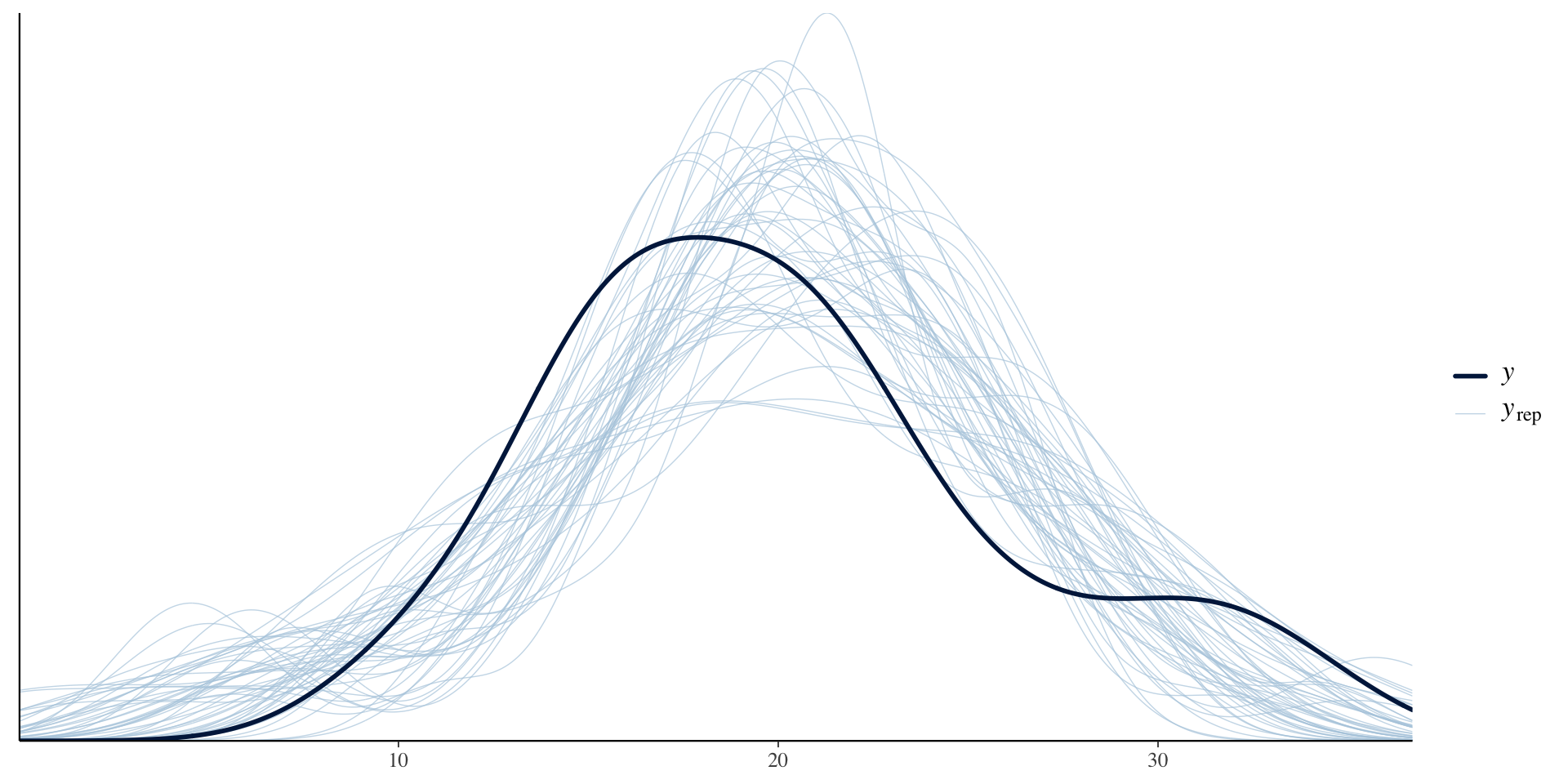
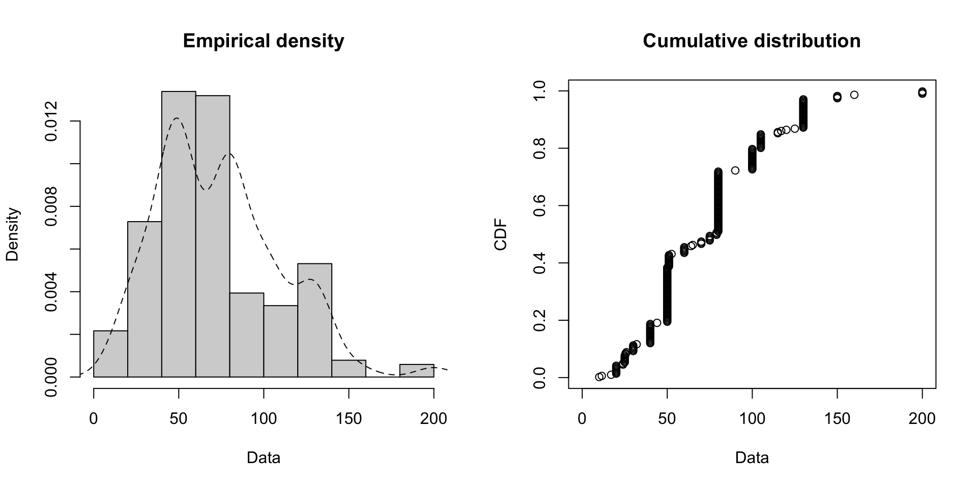
In other words, taking the data and fitting a distribution implies we think the data perfectly determines the distribution. This may not be (and often isn’t) the case.
For the purposes of this course the defaults will be fine.
One of the bigger challenges for non-statisticians like us is understanding the underlying assumptions and applicability of probability distributions. In a lot of cases the Normal, Poisson, logNormal distributions (in addition to Uniform) give us most of what we need for this course.
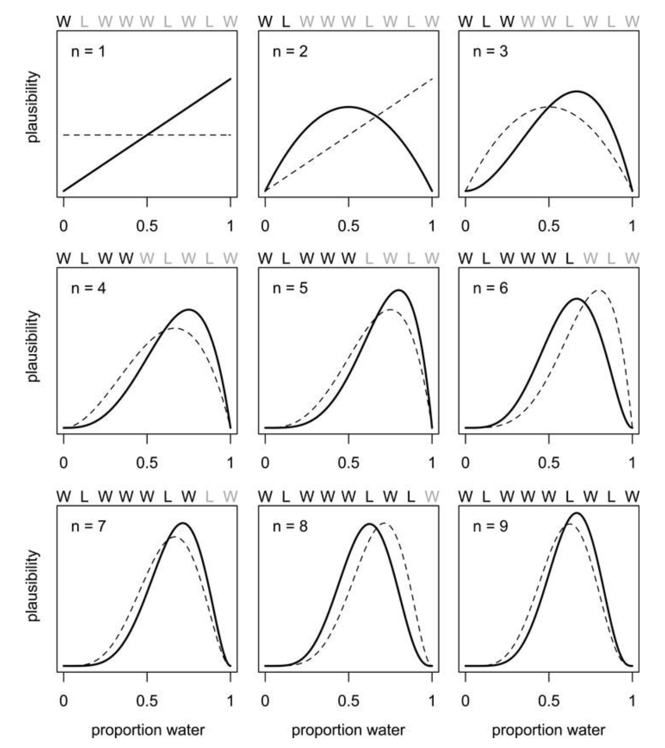
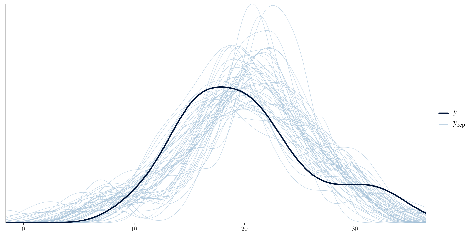
Effect of prior on data (and vice-versa)