Bayesian Data Analysis in SE

2025-07-29
Introduction
(This is mostly based on McElreath’s book)
McElreath has this notion of golem, essentially a mechanical device that for a given input produces some statistical test output. In our world these are the models we work with.

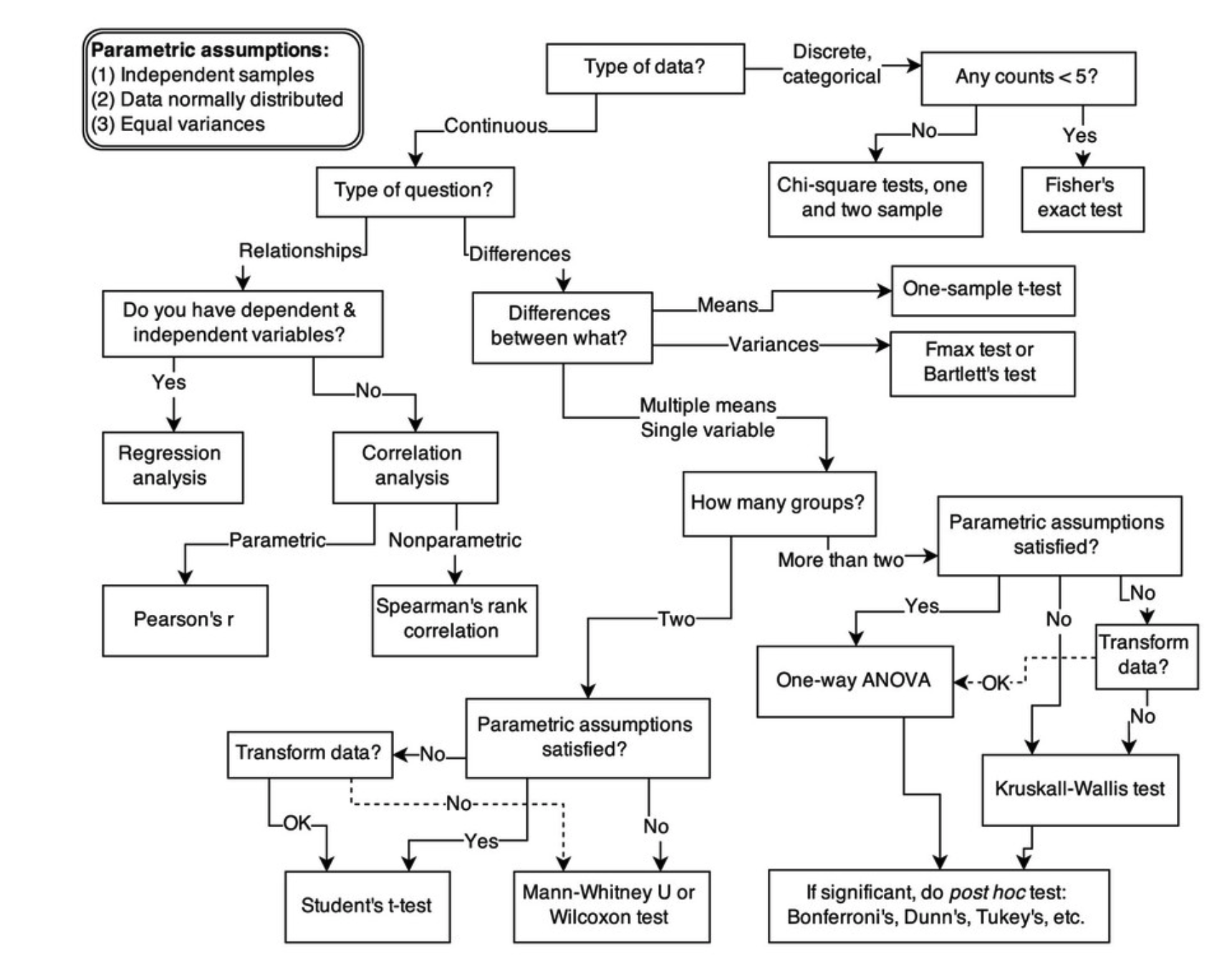
For example, if I have two sample populations with mean \(x_i\) and \(x_j\), st dev \(s_i,s_j\), then my golem might tell me to use a t-test to compare the means.
And importantly (hence the golem metaphor) without any awareness of what the inputs are, and especially with no idea if that is the right golem to use for the problem. Thus we should be very careful when relying only on statistical tests, as their results may not be accurate.
(and see also the “all tests are linear models” slide)
Golems in stats
(from Ch 1 of Stat. Rethinking)
Bayesian Data Analysis
Bayesian Analysis
Count all the ways data can happen under the assumptions. Assumptions with more ways the data can happen are more plausible.
Model plausibility: instead of falsifying some (often arbitrary and unrealistic) null hypothesis model (e.g., programming skill has NO EFFECT on task time), compare credible models (or hypotheses).
Which one best describes the data? Which one best predicts unseen data?
- Watch for overfitting - if we train on the data, the model knows the sample really well, but not the broader world (which is what we care about!)
- Use information theory (AIC, cross-validation) to compare
- AIC = error from model + penalty for having too many parameters (DoF)
Marbles example
- see McElreath, chapter 2
Bayes with marbles
A conjectured proportion of blue marbles, p, is usually called a PARAMETER value. It’s just a way of indexing possible explanations of the data.
The relative number of ways that a value p can produce the data is usually called a LIKELIHOOD. It is derived by enumerating all the possible data sequences that could have happened and then eliminating those sequences inconsistent with the data.
The prior plausibility of any specific p is usually called the PRIOR PROBABILITY.
The new, updated plausibility of any specific p is usually called the POSTERIOR PROBABILITY.
Bayesian inference: the ICSE example.
Then we can use Bayes’s law to say
Posterior probability is proportional to Probability of data X Prior probability
Exercise
What is happening in the code (see Github).
A Bayesian Workflow
- Pick a model
- Check the model and prior against domain knowledge
- Fit the model (e.g. call
ulam()orbrms()or similar) - Validate the computation/sampling: convergence diagnostics, r-hat
- Fix the computation - rewrite the model
- Evaluate and Use Model (predict, cross-validate, posterior predictive checks)
- Modify the model - new priors, more data, new predictors
- Compare models - leave-one-out information criterion, model averaging
Building Models
Note: we can write linear regression equations as either \(y = mx + b\) or as the model variant of that, \(y \sim Normal(\mu,\sigma)\) (and possibly some error term \(\epsilon\))
From Chapter 4.2 (a language for describing models):
- What measurements (variables) are we hoping to predict/understand? (\(y\), here)
- For each variable, what is a likelihood that describes the plausibility of the observations? (Here, Normal())
- What predictor variables will help us find the outcomes?
- Use these predictors to define the shape and location of the likelihood (here, \(\mu,\sigma\))
- Choose priors to define our initial information state for all model parameters. (Where should the mean be? What should sigma be? )
Statistical Model Specification in R and Stan
We now can specify our statistical model using the tilde notation. For variables W (for waistline), D (for Donuts), we can say W is influenced by / predicated by / modelled by D, i.e., donut consumption influences waist line. We write this as:
\(W \sim D\)
Translate it into Stan’s DSL (see 4.3):
Recall linear regression can be specified as
\(y_i \sim \mathcal{N}(\mu, \sigma)\)
and then model it using Stan.
Code
Running MCMC with 2 parallel chains, with 1 thread(s) per chain...

Chain 1 Iteration:   1 / 1000 [  0%]  (Warmup)
Chain 1 Iteration: 100 / 1000 [ 10%]  (Warmup)
Chain 1 Iteration: 200 / 1000 [ 20%]  (Warmup)
Chain 1 Iteration: 300 / 1000 [ 30%]  (Warmup)
Chain 1 Iteration: 400 / 1000 [ 40%]  (Warmup)
Chain 1 Iteration: 500 / 1000 [ 50%]  (Warmup)
Chain 1 Iteration: 501 / 1000 [ 50%]  (Sampling)
Chain 1 Iteration: 600 / 1000 [ 60%]  (Sampling)
Chain 1 Iteration: 700 / 1000 [ 70%]  (Sampling)
Chain 1 Iteration: 800 / 1000 [ 80%]  (Sampling)
Chain 1 Iteration: 900 / 1000 [ 90%]  (Sampling)
Chain 1 Iteration: 1000 / 1000 [100%]  (Sampling)
Chain 2 Iteration:   1 / 1000 [  0%]  (Warmup)
Chain 2 Iteration: 100 / 1000 [ 10%]  (Warmup)
Chain 2 Iteration: 200 / 1000 [ 20%]  (Warmup)
Chain 2 Iteration: 300 / 1000 [ 30%]  (Warmup)
Chain 2 Iteration: 400 / 1000 [ 40%]  (Warmup)
Chain 2 Iteration: 500 / 1000 [ 50%]  (Warmup)
Chain 2 Iteration: 501 / 1000 [ 50%]  (Sampling)
Chain 2 Iteration: 600 / 1000 [ 60%]  (Sampling)
Chain 2 Iteration: 700 / 1000 [ 70%]  (Sampling)
Chain 2 Iteration: 800 / 1000 [ 80%]  (Sampling)
Chain 2 Iteration: 900 / 1000 [ 90%]  (Sampling)
Chain 2 Iteration: 1000 / 1000 [100%]  (Sampling)
Chain 1 finished in 0.0 seconds.
Chain 2 finished in 0.0 seconds.

Both chains finished successfully.
Mean chain execution time: 0.0 seconds.
Total execution time: 0.2 seconds. mean sd 5.5% 94.5% rhat ess_bulk
mu 171.01692 7.819862 158.75339 183.14354 1.001740 509.2914
sigma 20.30586 7.019116 11.30596 33.97946 1.016116 246.2645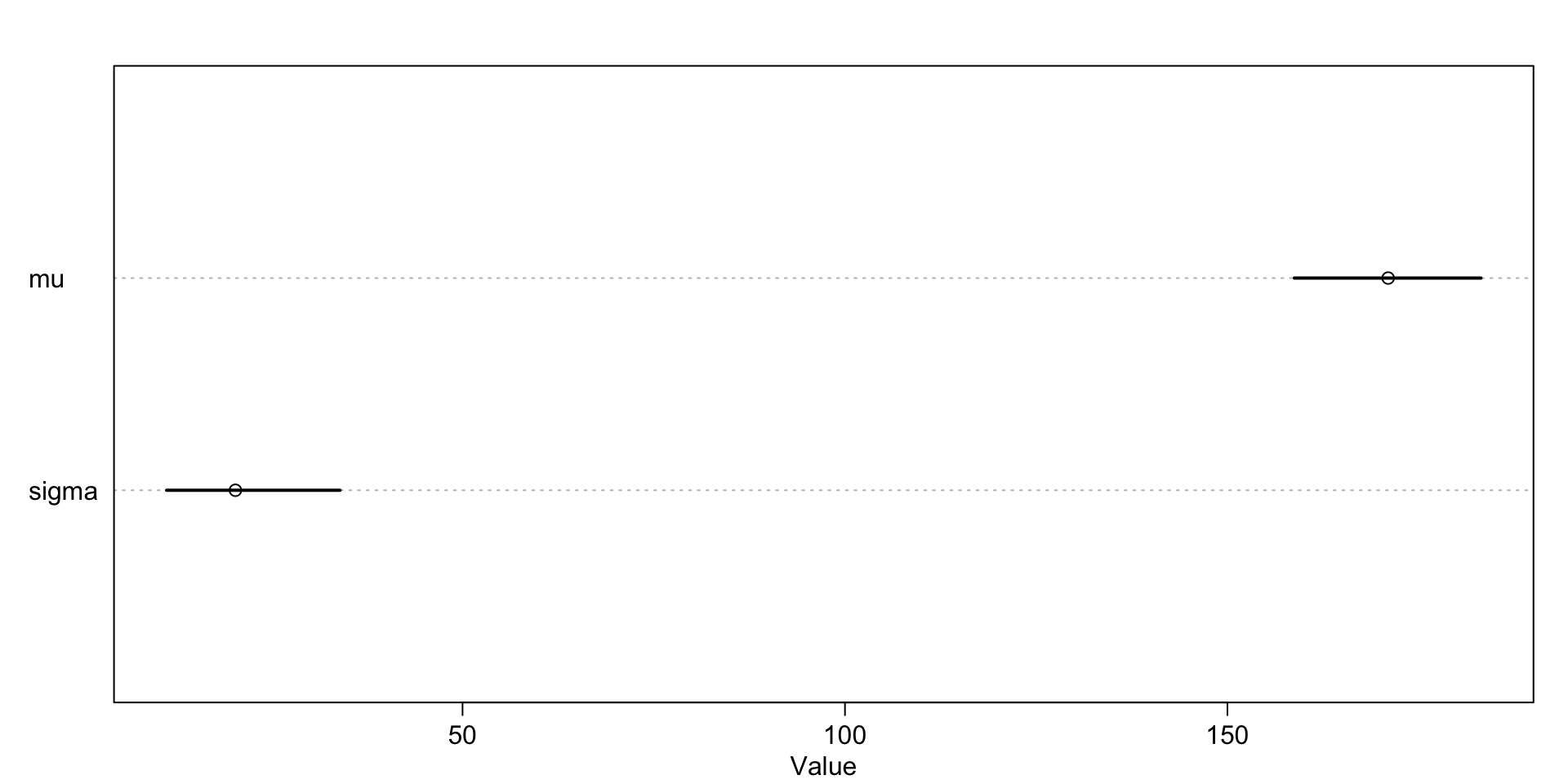
Summary
Bayesian modeling forces us to think about
- what weight to ascribe to past understanding of the phenomena (if any)
- what makes the observations likely to occur
- doing some sampling (HMC) to find the posterior probability distributions

Neil Ernst ©️ 2024-5