Linear Regression
2025-07-29
Regression
Regression basics
A useful approach, which we cover in Assignment 1, is to do a simple linear regression.
In the simplest sense this is about finding the line that best fits the data.
Extending the line to unseen datapoints is a prediction about what the y value should be for that data (a set of observations X).
Digression: Modeling
The word ‘model’ is overloaded in computer science (i.e., overused). Here, I will use it to mean statistical model, and it captures the intuition we discussed earlier: how we think the data are being generated. In this course I take the position that it is usually always possible to represent data with a simpler, more abstract model.
For example, obviously how each individual in this course got to be the height they are is subject to a vast array of forces, including genetics (the big one), nutrition, air pollution, etc.
Modeling
In data science, we would like to abstract all of this complexity at the individual level with an abstraction for the sample, and talk about averages, deviations, and assume that randomness in sufficiently large numbers 1 will take care of the individual variation.
Another approach is to throw up our hands and forget about representing the data using an underlying generative model, and instead fit functions of high dimensionality to represent the way the data is distributed, the neural approach. We will see both in this course.
OLS regression
Ordinary least squares (OLS) regression is possible when there is a simple relationship to plot.
It looks like: \(y_i = \beta x_i + \alpha + \epsilon_i\)
And our task is to find \(\alpha, \beta\) to minimize the (squared) error in our estimated \(\hat{y}\), i.e. the value \(y_i - \hat{y}\) for all the \(y\) s.
If we think about y as predicting bug count/defects h, we can simply say your file’s bugginess is some intercept \(\alpha\) and an error term. The error term \(\epsilon\) here is capturing things like the inherent error in our measurements (if we are measuring 100 files, we might get sloppy).
This regression equation has a precise (algebraic) solution using the ordinary least squares technique.
An alternative representation uses the Gaussian model which captures the intuition that the residuals (difference between estimate and actual) are normally distributed about the mean:
\(y_i \sim \mathcal{N}(\mu, \sigma)\)
\(\mu \sim Normal(param, param)\)
\(\sigma \sim\) Uniform(param, param)
This equation says that our data point \(y_i\) is modeled by (the \(\sim\) or tilde operator) a Normal distribution with location (mean) \(\mu\) and dispersion (variance) \(\sigma\). The next two lines are where we might specify our prior about how the location and dispersion should be defined.
The generalized version of this is a generalized linear model or GLM, and accounts for things like how the data and the marginals (the error) are distributed, as we saw in A1.
R has a built in function, glm() (for generalized linear model) that is frequentist:
Let’s break this down a bit.
The first part is the defects ~ loc notation. This is R’s way of encoding the statistical model. In this case, we are saying that the response in whether the row has defect=True is modeled by the loc (lines of code) feature (predictors).
We could maybe write defects ~ loc + v(g). These are two separate models; the two include linear predictors with no interactions. Special variants include defects ~ . (all predictors) and defects ~ 1 (no predictors).
Finally, we have a parameter family=binomial. This parameter is saying that for this regression model, the sampler (in this case, a maximum likelihood estimation (MLE, a variant of Newton’s method)) should do logistic regression and predict a binary outcome. Both logistic and linear regression are variants of generalized linear models.
Interpreting Regression Results
(see also ROS, chapter 6.3, and chapter 10, p133)
We now have a model fit object fit that we will want to explore. Hopefully, we will see that it fits the equation for a linear model we mentioned above, with intercepts and coefficients:
Call:
glm(formula = defects ~ loc, family = binomial, data = jm1)

Coefficients:
             Estimate Std. Error z value Pr(>|z|)
(Intercept) -1.937164   0.033757  -57.39   <2e-16 ***
loc          0.010859   0.000466   23.30   <2e-16 ***
---
Signif. codes:  0 '***' 0.001 '**' 0.01 '*' 0.05 '.' 0.1 ' ' 1

(Dispersion parameter for binomial family taken to be 1)

    Null deviance: 10687.4  on 10882  degrees of freedom
Residual deviance:  9954.1  on 10881  degrees of freedom
AIC: 9958.1

Number of Fisher Scoring iterations: 5
This prints out coefficient on the predictor (‘m’) and the intercept (that’s the b in the y=mx + b + e notation). The second column reflects the uncertainty in the estimate. So what do we make of this? The first thing we should do is print out one of the interactions:
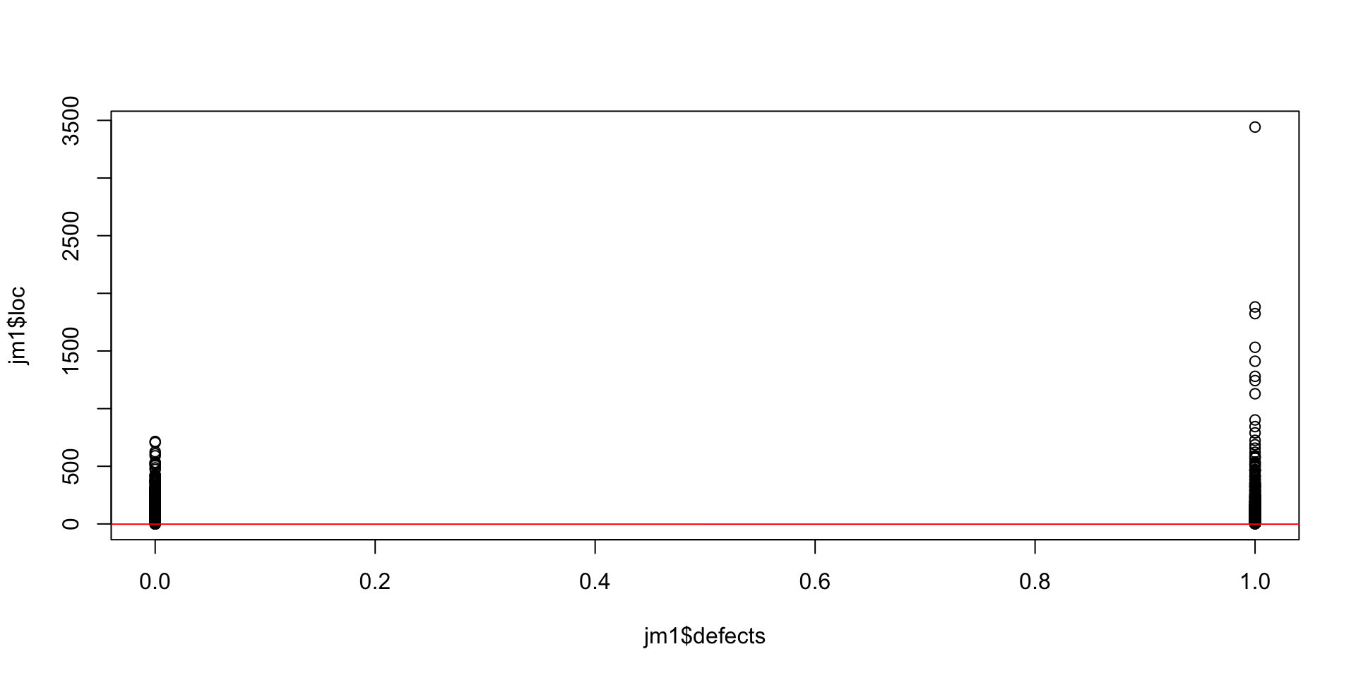
Here we have our two values for defective files, and the LOC on the y-axis.
A red line indicates the regression equation that fits this data using OLS. From our fit_1 object, we can see the intercept is b=-1.9, and m is 0.01 (the slope of the red line).
Recall our model: we think (or, we are testing), the idea that if code has more lines, it is more likely to have defects.
So what this model predicts is that the change in lines of code increases ‘defect’ likelihood by 0.01 (1%) of the number of lines.
This corresponds to a defect rate of 1 bug per 100 lines of code, which is actually pretty close to reports: Microsoft at one point estimated 10-20 defects per 1000 LOC 1
A few issues to note here:
- coefficients represent the mean change in the dependent variable for each 1 unit change in an independent variable when you hold all of the other independent variables constant.
- this is just one model, and if we follow our workflow, we should now be comparing this model to others, which might be changes to this one, or adding new features.
- we have a negative intercept, which makes no sense because we can’t have negative LOC. We would want to fix that in our revised model.
- we have a lot of data distributed around the 1-100 LOC mark. We should adjust our model (at the very least, our visualization) to accommodate this non-normal distribution.
- some of our files have NO bugs, and these “zeros” are inflating the estimates.
Bayesian regression
From a Bayesian point of view we can use the rstanarm library, which is the same format as the glm() command, but uses a Bayesian interpretation and sampler:
A bunch of text should fly by in the console; this is the sampler running on the likelihood.
Happily (I think you would agree) the Bayesian approach finds similar parameters as the frequentist/MLE approach before.
You might say “the outputs of both of these approaches are very similar” and thus, who cares if it is frequentist.
Pragmatically I suppose that is true but you can get into trouble in the edges.
In some sense we would hope that two different inferential approaches will find the same outcomes, if that outcome is a real thing.
| Bayes | Frequentist |
|---|---|
| Prior captures past knowledge | Assumption of ignorance about past |
| Sample from likelihood | Maximum likelihood estimation (MLE) |
| Computationally more costly | usually cheap |
| Posterior represents probability of the parameter being true | p-value captures likelihood of observing data as extreme or more so, under null hypothesis |
Model Comparison and Evaluation
For the frequentist linear regression approach, we have a metric such as \(R^2\), which measures the goodness of fit or proportion of variance explained.
A perfect linear model would have \(R^2\) of 1.0, indicating all the variance in the data is captured in the model.
Call:
lm(formula = m1, data = mtcars)

Residuals:
    Min      1Q  Median      3Q     Max
-5.7121 -2.1122 -0.8854  1.5819  8.2360

Coefficients:
            Estimate Std. Error t value Pr(>|t|)
(Intercept) 30.09886    1.63392  18.421  < 2e-16 ***
hp          -0.06823    0.01012  -6.742 1.79e-07 ***
---
Signif. codes:  0 '***' 0.001 '**' 0.01 '*' 0.05 '.' 0.1 ' ' 1

Residual standard error: 3.863 on 30 degrees of freedom
Multiple R-squared:  0.6024,    Adjusted R-squared:  0.5892
F-statistic: 45.46 on 1 and 30 DF,  p-value: 1.788e-07
Code
         fit       lwr       upr
1 13.0417910 10.491571 15.592011
2  9.6303771  6.168609 13.092145
3 -0.6038646 -7.025504  5.817775
For our fit_1 object above, which is a logistic regression model, a better measure is the classification accuracy (defective/not defective).
We can use the model’s fitted values (fit_1$fitted.values) to compare. I’m not an expert in this, however.
The Bayesian intuition
Having a Bayesian model is helpful in capturing an intuition about the data.
It produces a fit object that is really a posterior probability distribution that gives us the ability to do stuff like sample from it, retrieve arbitrary intervals, etc.
As Regression and Other Stories notes (p. 99), we should interpret the coefficients as comparisons.
We can say that, under the fitted model, the average difference in earnings, comparing two people of the same sex but one inch different in height, is $600. The safest interpretation of a regression is as a comparison (emphasis added)
Similarly, in our case we are implicitly comparing two files, with 100 lines of code difference, we would expect an increase of one defect.
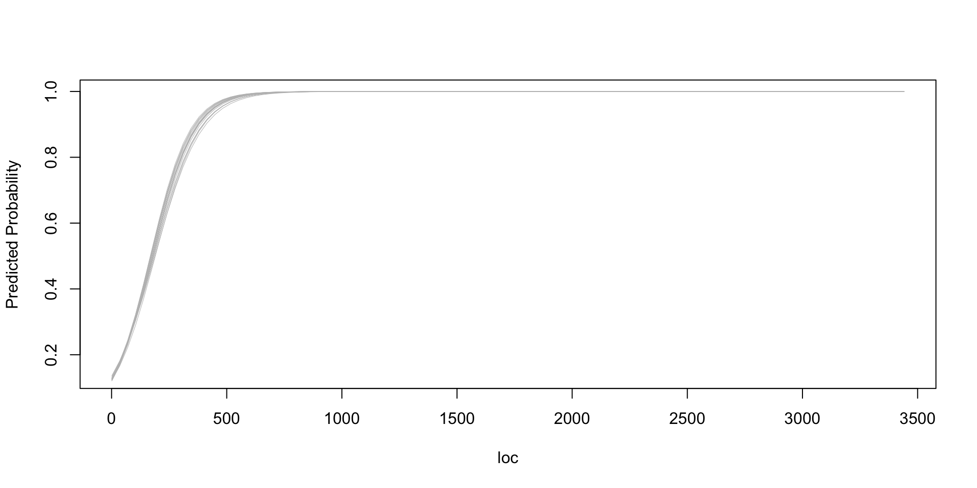
Code
plot.new()
x <- seq(min(jm1$loc, na.rm=TRUE), max(jm1$loc, na.rm=TRUE), length.out=100)
sims_1 <- as.matrix(fit_b)
n_sims <- nrow(sims_1)
plot(x, invlogit(sims_1[1,1] + sims_1[1,2]*x), type="n", xlab="loc", ylab="Predicted Probability")
for (j in sample(n_sims, 20)){
    curve(invlogit(sims_1[j,1] + sims_1[j,2]*x), from=min(x), to=max(x), col="gray", lwd=0.5, add=TRUE)
}
Overfitting
One problem is that a model with 8 datapoints is perfectly explained by 8 variables.
This overfitting issue can occur in regression as well, if we have models - like this jm1 dataset - with many variables.
It also makes interpretation harder, as we have to explain the outputs based on more of these inputs.
Thus we might penalize the regression model to prevent overfitting and reward simpler models. Two such approaches are ridge and lasso regression.
Summary
- Regression is a core inferential tool in both frequentist and bayesian settings
- Very common in many other disciplines!
- Careful attention to the assumptions and interpretations of the coefficients - as comparisons - is key.

Neil Ernst ©️ 2024-5